问题背景 电力系统负荷(电力需求量,即有功功率)预测是指充分考虑历史的系统负荷、经济状况、气象条件和社会事件等因素的影响,对未来一段时间的系统负荷做出预测。负荷预测是电力系统规划与调度的一项重要内容。短期(两周以内)预测是电网内部机组启停、调度和运营计划制定的基础;中期(未来数月)预测可为保障企业生产和社会生活用电,合理安排电网的运营与检修决策提供支持;长期(未来数年)预测可为电网改造、扩建等计划的制定提供参考,以提高电力系统的经济效益和社会效益。
复杂多变的气象条件和社会事件等不确定因素都会对电力系统负荷造成一定的影响,使得传统负荷预测模型的应用存在一定的局限性。同时,随着电力系统负荷结构的多元化,也使得模型应用的效果有所降低,因此电力系统负荷预测问题亟待进一步研究。
需要解决的问题 1. 地区负荷的中短期预测分析 根据附件中提供的某地区电网间隔 15 分钟的负荷数据,建立中短期负荷预测模型:
给出该地区电网未来 10 天间隔 15 分钟的负荷预测结果,并分析其预测精度;(短期预测)
给出该地区电网未来 3 个月日负荷的最大值和最小值预测结果,以及相应达到负荷最大值和最小值的时间,并分析其预测精度。(中期预测)
2. 行业负荷的中期预测分析 对不同行业的用电负荷进行中期预测分析,能够为电网运营与调度决策提供重要依据。特别是在新冠疫情、国家“双碳”目标等背景下,通过对大工业、非普工业、普通工业和商业等行业的用电负荷进行预测,有助于掌握各行业的生产和经营状况、复工复产和后续发展走势,进而指导和辅助行业的发展决策。请根据附件中提供的各行业每天用电负荷相关数据,建立数学模型研究下面问题:
挖掘分析各行业用电负荷突变的时间、量级和可能的原因。 给出该地区各行业未来 3 个月日负荷最大值和最小值的预测结果,并对其预测精度做出分析。 根据各行业的实际情况,研究国家“双碳”目标对各行业未来用电负荷可能产生的影响,并对相关行业提出有针对性的建议。 解题过程 主办方提供的数据量虽然非常多,但由于受到机器学习硬件的限制,显然不能将其直接投喂进去。并且还需要对数据进行统合整理,只将需要的数据投入。
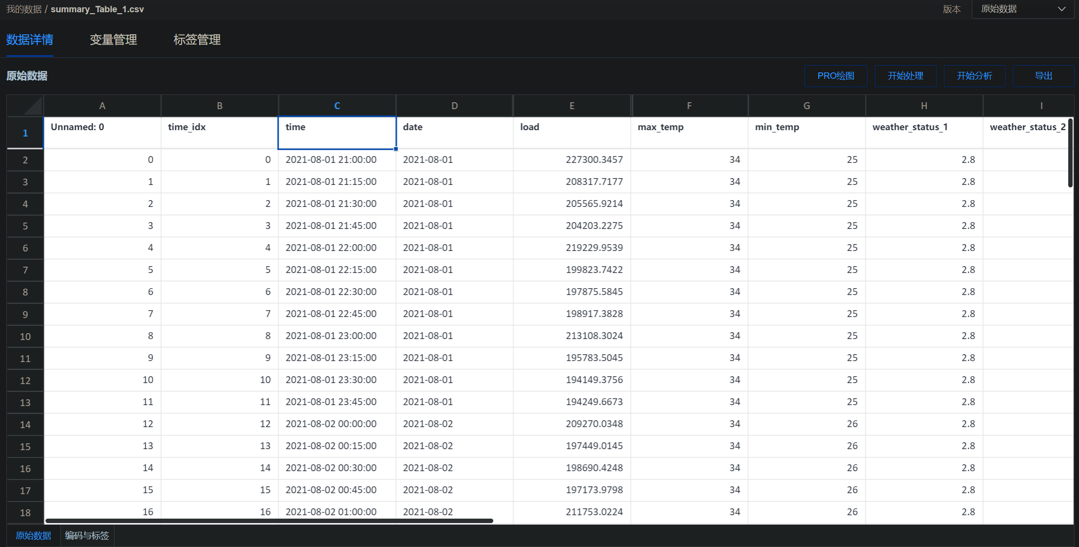
数据处理 历史负荷数据处理 在对历史 15 分钟间隔的负荷数据处理时,需要将原本的时间数据转换为 Timestamp 类型,存入time列。同时由于其他文件中的时间并没有具体的时间只有日期,因此也需要将他们的日期标注出来,放在date列当中。
1
2
3
4
5
6
7
8
9
10
11
12
13
14
15
16
raw_load_data = raw_load_data.tail(训练集大小*30 *96 ) raw_load_data.reset_index(drop=True , inplace=True ) slicing = raw_load_data.join( raw_load_data["数据时间" ].str .split(" " , expand=True )) raw_load_data["date" ] = slicing[0 ] raw_load_data["date" ] = pandas.to_datetime(raw_load_data["date" ]) raw_load_data["date" ] = pandas.DatetimeIndex(raw_load_data["date" ]).date raw_load_data["time" ] = pandas.to_datetime(raw_load_data["数据时间" ]) raw_load_data['time_idx' ] = raw_load_data.index raw_load_data["数据时间" ] = pandas.to_datetime(raw_load_data["数据时间" ])
天气数据处理 天气数据分别有:
最高气温 最低气温 白天风向 夜间风向 白天风速 夜间风速 天气状况 1 天气状况 2 首先为天气数据添加时间序列。并且对气温进行处理,使其为 int 型。最后将天气状况以“/”为分隔符进行分割,生成"天气状况 1"与"天气状况 2"列。
1 2 3 4 5 6 7 8 9 10 11 12 13 raw_climate_data["日期" ] = pandas.to_datetime( raw_climate_data["日期" ], format ="%Y年%m月%d日" ) raw_climate_data["最高温度" ] = raw_climate_data["最高温度" ].map ( lambda str : int (str .replace("℃" , "" ))) raw_climate_data["最低温度" ] = raw_climate_data["最低温度" ].map ( lambda str : int (str .replace("℃" , "" ))) slicing = raw_climate_data.join( raw_climate_data["天气状况" ].str .split("/" , expand=True )) raw_climate_data["天气状况 1" ] = slicing[0 ] raw_climate_data["天气状况 2" ] = slicing[1 ]
在将天气状况切分之后,检查都有哪些天气类型
1 2 3 4 5 6 7 8 raw_climate_data["天气状况 1" ] = raw_climate_data["天气状况 1" ].map ( lambda str : str .replace("到" , "雨-" )) raw_climate_data["天气状况 2" ] = raw_climate_data["天气状况 2" ].map ( lambda str : str .replace("到" , "雨-" )) raw_climate_data["天气状况 1" ].unique() raw_climate_data["天气状况 2" ].unique()
1
2
array(['多云', '阴', '小雨', '中雨-大雨', '中雨', '小雨-中雨', '晴', '局部多云', '阵雨', '雾', '雷阵雨', '大雨', '暴雨', '大雨-暴雨'], dtype=object)
可以发现有下列几种:
多云 阴 小雨 中雨 - 大雨 中雨 小雨 - 中雨 晴 局部多云 阵雨 雾 雷阵雨 大雨 暴雨 大雨 - 暴雨 对数据进行标记:
1 2 3 4 5 6 7 8 9 10 11 12 13 14 15 16 17 18 19 20 weather = { "晴" : 0 , "局部多云" : 0.5 , "多云" : 1 , "阴" : 2 , "雾" : 2.2 , "阵雨" : 2.5 , "雷阵雨" : 2.8 , "小雨" : 3 , "小雨 - 中雨" : 3.5 , "中雨" : 4 , "中雨 - 大雨" : 4.5 , "大雨" : 5 , "大雨 - 暴雨" : 5.5 , "暴雨" : 6 , } raw_climate_data["天气状况 1" ] = raw_climate_data["天气状况 1" ].map (weather) raw_climate_data["天气状况 2" ] = raw_climate_data["天气状况 2" ].map (weather)
而对于风向风力数据,由于其中所使用的连接字符并不统一,因此需要先将其统一为-再对风向风力数据进行去重。
1 2 3 4 5 6 7 raw_climate_data["白天风力风向" ] = raw_climate_data["白天风力风向" ].map ( lambda str : str .replace("~" , "-" )) raw_climate_data["夜晚风力风向" ] = raw_climate_data["白天风力风向" ].map ( lambda str : str .replace("~" , "-" )) raw_climate_data["白天风力风向" ].unique() raw_climate_data["夜晚风力风向" ].unique()
1
2
3
4
array(['无持续风向<3级', '北风4-5级', '微风<3级', '北风3', '东北风3-4级', '北风3-4级', '南风3-4级', '南风4-5级', '东北偏东风2', '无持续风向微风', '无持续风向1-2级', '东风3-4级', '东南风4-5级', '东风8-9级', '东南风3-4级', '南风1-2级', '东南风1-2级', '西南风3-4级', '东风1-2级', '北风1-2级', '东北风1-2级', '西南风1-2级'], dtype=object)
在去重之后,可以发现一共有 23 种风力风向类型:
无持续风向<3 级 北风 4-5 级 微风<3 级 北风 3 东北风 3-4 级 北风 3-4 级 南风 3-4 级 南风 4-5 级 东北偏东风 2 无持续风向微风 无持续风向 1-2 级 东风 3-4 级 东南风 4-5 级 东风 8-9 级 东南风 3-4 级 南风 1-2 级 东南风 1-2 级 西南风 3-4 级 东风 1-2 级 北风 1-2 级 东北风 1-2 级 西南风 1-2 级 因为连在一起标记不太能体现出特征,因此将风力与风向特征分开标记。
1 2 3 4 5 6 7 8 9 10 11 12 13 14 15 16 17 18 19 20 21 22 23 24 25 26 27 28 29 30 31 32 33 34 35 36 37 38 39 40 41 42 43 44 45 46 47 48 49 50 wind_direction = { "无持续风向" : 0 , "北风" : 1 , "南风" : 2 , "西风" : 3 , "东风" : 4 , "东北风" : 5 , "东南风" : 6 , "西南风" : 7 , "西北风" : 8 , "东北偏东风" : 9 , } wind_power = { "1-2 级" : 1.5 , "2" : 2 , "<3 级" : 2.5 , "微风" : 3 , "3" : 3 , "3-4 级" : 3.5 , "4-5 级" : 4.5 , "8-9 级" : 8.5 , } import redef direction (str miao = re.search("无持续风向 | 东北偏东风|[^微]{1,2}风" , str , flags=0 ) if miao == None : return 0 return wind_direction[miao.group()] def power (str miao = re.search("[^-]\d级|\d-\d级|\d|微风" , str , flags=0 ) return wind_power[miao.group()] raw_climate_data["wind_direction_1" ] = raw_climate_data["白天风力风向" ].map ( lambda str : direction(str )) raw_climate_data["wind_direction_2" ] = raw_climate_data["夜晚风力风向" ].map ( lambda str : direction(str )) raw_climate_data["wind_power_1" ] = raw_climate_data["白天风力风向" ].map ( lambda str : power(str )) raw_climate_data["wind_power_2" ] = raw_climate_data["夜晚风力风向" ].map ( lambda str : power(str ))
至此,天气的数据已经标记完成。
数据合并 数据处理完成后,将两张表的数据合并到同一张总表上
1 2 3 4 5 6 7 8 9 10 11 12 13 14 15 16 summary_Table = pandas.DataFrame() summary_Table["time_idx" ] = raw_load_data["time_idx" ] summary_Table["time" ] = raw_load_data["time" ] summary_Table["date" ] = raw_load_data["date" ] summary_Table["load" ] = raw_load_data["总有功功率(kw)" ] source = ["最高温度" , "最低温度" , "天气状况 1" , "天气状况 2" , "wind_direction_1" , "wind_direction_2" , "wind_power_1" , "wind_power_2" ] target = ["max_temp" , "min_temp" , "weather_status_1" , "weather_status_2" , "wind_direction_1" , "wind_direction_2" , "wind_power_1" , "wind_power_2" ] for i in target: summary_Table[i] = summary_Table["date" ].map ( lambda date: raw_climate_data[source[target.index(i)]].loc[raw_climate_data["日期" ] == date.strftime("%Y-%m-%d" )].values[0 ]) summary_Table["group" ] = numpy.zeros(summary_Table.shape[0 ])
为了方便对数据进行多时长的提取分析处理,将上述数据处理过程统合为了一个数据处理脚本,方便随时调用。
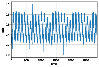
数据分析 为了分析负荷数据在时间上呈现何种分布,我们先是提取出最新的一个月的数据
1 python ./数据处理.py --length 1 --name "summary_Table_1.csv"
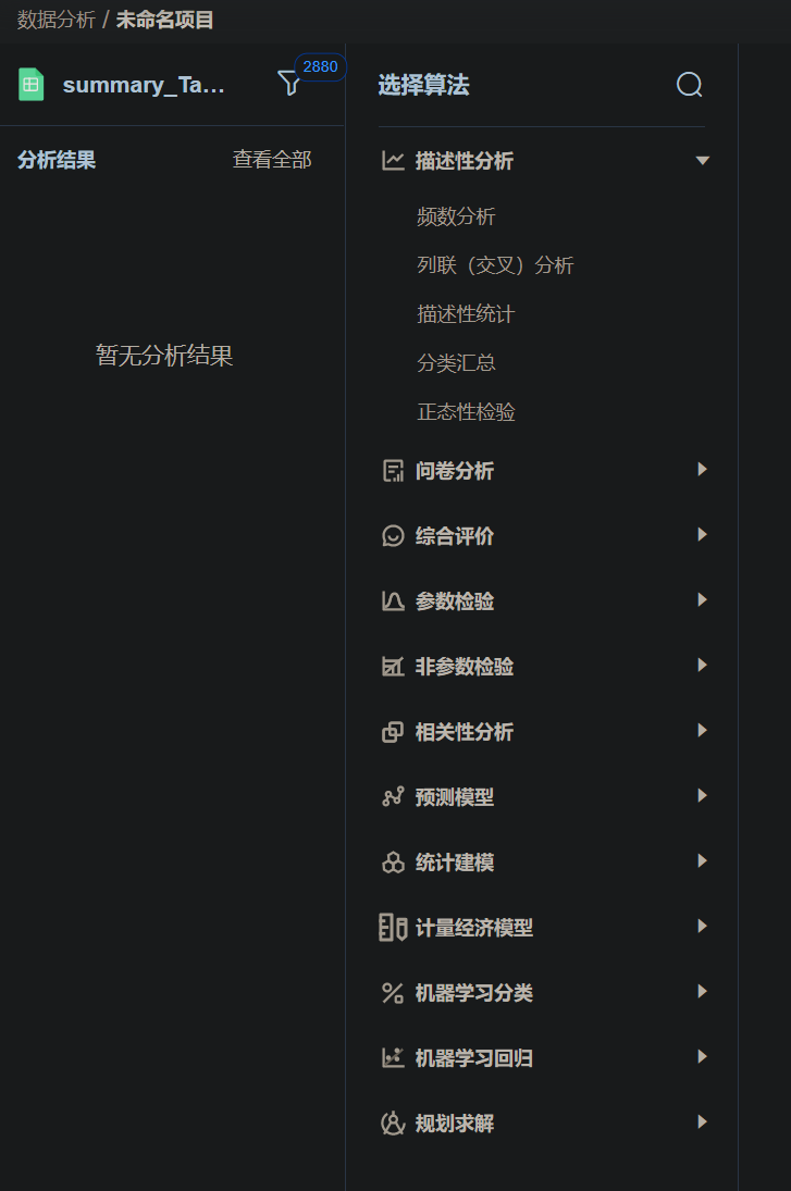
随后将数据上传到 SPSSPRO 数据分析平台上。
SPSSPRO 是众言科技旗下的一款集专业统计方法与数据算法于一体的免费在线数据分析平台。可实现异常值检验、样本均衡、数据降维等多种数据处理方式。涵盖全部专业统计 SPSS 算法模型,已开发 200 余种算法,可做统计分析(如 T 检验等)、综合评价(如层次分析,数据包络等)、机器学习时间序列等等,一键生成分析与解释,小白也能看懂分析报告。
点击右上方的开始分析按钮,进入数据分析页面
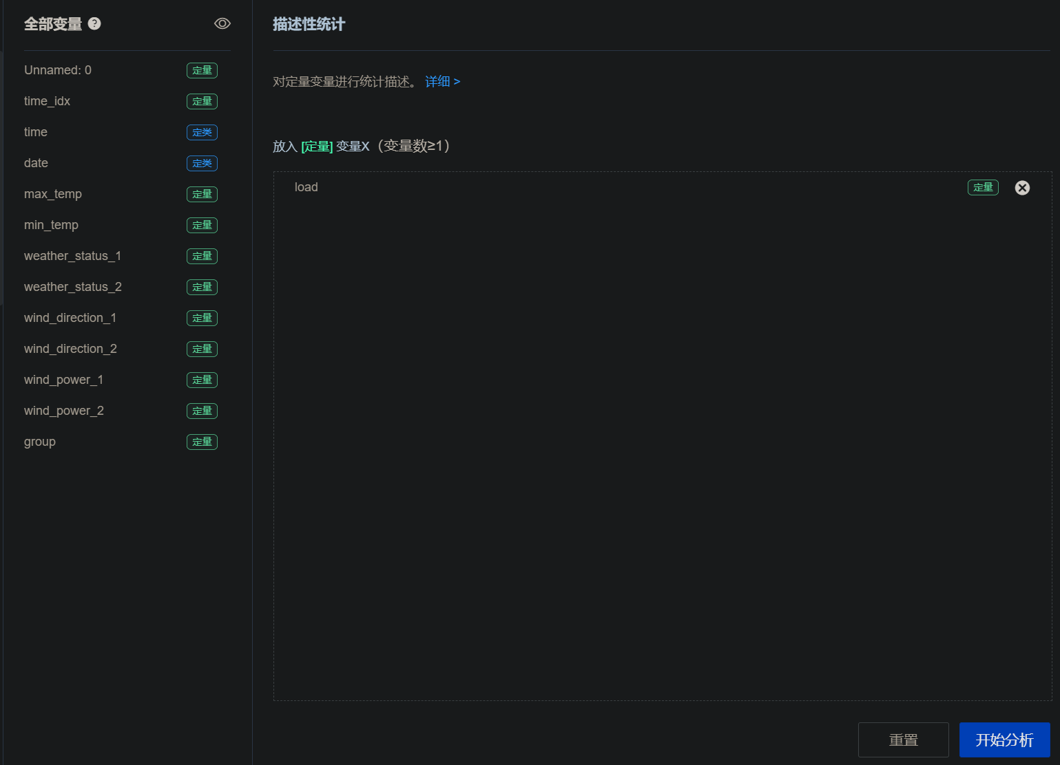
可以看见 SPSSPRO 数据分析平台拥有种类繁多的分析项目,让零基础的机器学习小白也能轻松入门。这次我使用描述性分析-描述性统计功能分析数据。
在将需要分析的定量拖入右侧后,点击下方的开始分析后便能马上得到分析结果了。
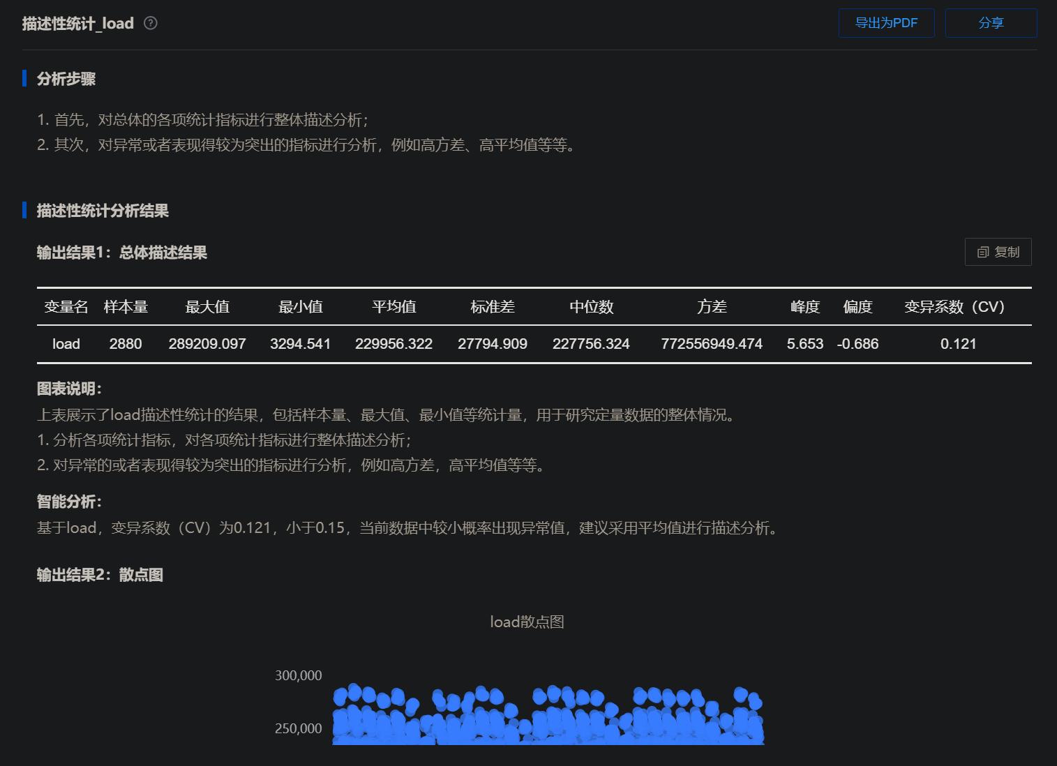
从分析结果中我们可以看见,该负荷在过去的一个月中最大值为 289209.097(kw),最低为 3294.541(kw)。为什么最高值与最低值会差别那么大呢,难道是用电量的波动较大吗?如果是过去,可能就需要将图表画出来再根据图像进行分析了,但 SPSSPRO 数据分析平台还有智能分析的功能:下面给出的智能分析中可以知道,这个 3294.541(kw)的最低值应该为异常值,并且是小概率出现的。因此在后面的构建模型的过程中需要将其处理后才能使用。
异常值处理 对异常值的处理大致上可以分为三种,分别是:设为缺失值、填补、不处理。
置空
将异常数据设置为 Null 值。此类处理最简单,而且绝大多数情况下均使用此类处理;直接将异常值删除,相当于没有该异常值。如果异常值不多时建议使用此类方法。
填补
如果异常值非常多时,则可能需要进行填补设置,SPSSAU 共提供平均值,中位数,众数和随机数、填补数字 0 共五种填补方式。
不处理
一些异常值也可能同时包含有用的信息,是否需要剔除,应由分析人员自行判断。
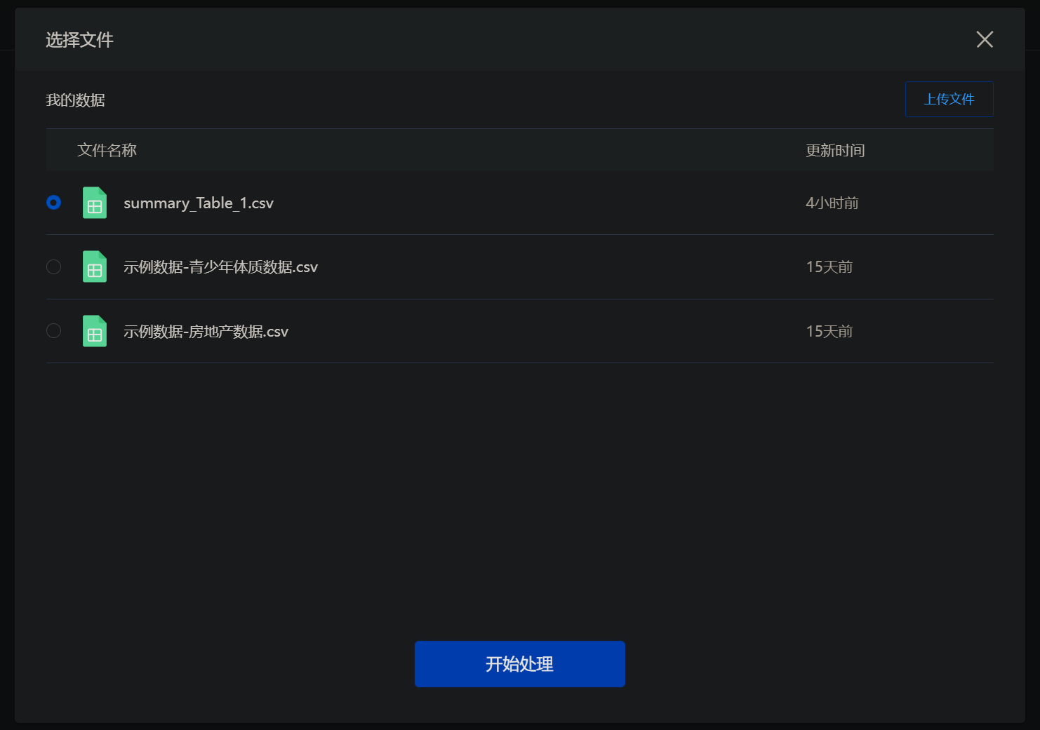
这里我们可以使用 SPSSPRO 数据分析平台提供的数据处理功能来对上面得到的异常值进行处理。首先点击上方的数据处理,然后新建一个处理
在弹出的窗口中选中需要处理的文件,点击开始处理
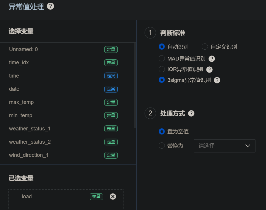
将load拖入下方后,在右边选择 3slgma 异常值识别,处理方式选择置为空值。
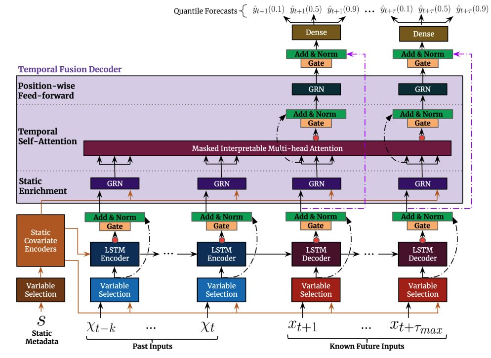
模型构建与训练 由上面的数据分析部分可以知道,每日的 15 分钟间隔用电总有功功率是随着时间周期性浮动的,大致上呈现为一个平稳序列(stationary series),同时包含有季节(seasonality)成分。因此在模型的选择上,我们采用了在 2019 年由谷歌提出的 Temporal Fusion Transformers 算法模型。下图为 TFT 模型的架构:
建立数据集 导入经过处理的数据,并且将其归一化
1
2
3
4
5
6
7
8
9
10
11
12
13
14
15
16
17
18
19
20
21
22
23
24
25
26
27
import pandasimport matplotlib.pyplot as pltsummary_Table = pandas.read_csv(path) climate = ["max_temp" , "min_temp" , "weather_status_1" , "weather_status_2" , "wind_direction_1" , "wind_direction_2" , "wind_power_1" , "wind_power_2" ] for i in climate: summary_Table[i] = summary_Table[i].apply("str" ) summary_Table["time" ] = pandas.to_datetime(summary_Table["time" ]) summary_Table["date" ] = pandas.to_datetime(summary_Table["date" ]) max = summary_Table["load" ].max ()min = summary_Table["load" ].min ()summary_Table["load" ] = summary_Table["load" ].map ( lambda data: (data-min )/(max -min )) summary_Table.to_csv("out.csv" , index=False ) plt.title('' ) plt.ylabel('load' ) plt.xlabel('time' ) plt.grid(True ) plt.autoscale(axis='x' , tight=True ) plt.plot(summary_Table["load" ])
然后对短期的预测模型创建数据集
1
2
3
4
5
6
7
8
9
10
11
12
13
14
15
16
17
18
19
20
21
22
23
24
25
26
27
28
29
30
31
32
33
34
35
36
37
38
from pytorch_forecasting import TimeSeriesDataSetmax_step_length = 7 max_encoder_length = (96 *max_step_length) max_prediction_length = (predicted*96 ) training_cutoff = summary_Table["time_idx" ].max () - max_prediction_length datasets = TimeSeriesDataSet( summary_Table[lambda x: x.time_idx <= training_cutoff], time_idx='time_idx' , target="load" , time_varying_known_reals=["time_idx" ], time_varying_unknown_reals=["load" ], group_ids=["group" ], max_encoder_length=max_encoder_length, max_prediction_length=max_prediction_length, add_relative_time_idx=True , add_target_scales=True , add_encoder_length=True , ) validation = TimeSeriesDataSet.from_dataset( datasets, summary_Table, min_prediction_idx=datasets.index.time.max () + 1 , stop_randomization=True ) batch_size = batch train_dataloader = datasets.to_dataloader( train=True , batch_size=batch_size, num_workers=0 ) val_dataloader = validation.to_dataloader( train=False , batch_size=batch_size * 10 , num_workers=0 )
创建基线模型 1 2 3 4 actuals = torch.cat([y for x, (y, weight) in iter (val_dataloader)]) baseline_predictions = Baseline().predict(val_dataloader) (actuals - baseline_predictions).abs ().mean().item()
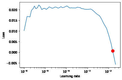
获取最佳学习率 在进行模型训练之前,还需要获取一个适用于该数据集于模型的最佳学习率。在机器学习和统计中,学习速率是优化算法中的调整参数,该优化算法可确定每次迭代时的步长,同时使损失函数趋于最小。
这里使用 PyTorch Lightning 中提供的 Learning Rate Finder 类来获得最佳的学习率。
1 2 3 4 5 6 7 8 9 10 11 12 13 14 15 16 17 18 19 20 21 22 23 24 25 26 27 28 29 30 31 32 33 34 35 36 37 38 39 40 41 42 43 44 import pytorch_lightning as plfrom pytorch_forecasting import QuantileLoss, DeepARpl.seed_everything(233 ) if accelerated == "gpu" : trainer = pl.Trainer( gpus=-1 , gradient_clip_val=0.1 , ) elif accelerated == "tpu" : trainer = pl.Trainer( tpu_cores=8 , gradient_clip_val=0.1 , ) else : trainer = pl.Trainer( gradient_clip_val=0.1 , ) module = DeepAR.from_dataset( datasets, learning_rate=0.03 , hidden_size=16 , dropout=0.1 , reduce_on_plateau_patience=4 , ) print (f"网络中的参数数量:{module.size()/1e3 :.1 f} k" )res = trainer.tuner.lr_find( module, train_dataloaders=train_dataloader, val_dataloaders=val_dataloader, max_lr=10.0 , min_lr=1e-6 , ) print (f"最佳的学习率:{res.suggestion()} " )optimal_learning_rate = res.suggestion() fig = res.plot(show=True , suggest=True ) fig.show()
最后得到如下的学习率曲线
此时程序输出的学习率为:0.01584893192461113
训练模型 1 2 3 4 5 6 7 8 9 10 11 12 13 14 15 16 17 18 19 20 21 22 23 24 25 26 27 28 29 30 31 32 33 34 35 36 37 38 39 40 41 42 43 44 45 46 47 48 49 50 51 52 53 54 55 56 57 58 59 60 61 62 63 64 65 66 67 68 from pytorch_lightning.callbacks import EarlyStopping, LearningRateMonitorfrom pytorch_lightning.loggers import TensorBoardLoggerearly_stop_callback = EarlyStopping( monitor="val_loss" , min_delta=1e-4 , patience=10 , verbose=False , mode="min" ) lr_logger = LearningRateMonitor() logger = TensorBoardLogger("lightning_logs" ) if accelerated == "gpu" : trainer = pl.Trainer( gpus=-1 , gradient_clip_val=0.1 , limit_train_batches=30 , callbacks=[lr_logger, early_stop_callback], logger=logger, ) elif accelerated == "tpu" : trainer = pl.Trainer( tpu_cores=8 , gradient_clip_val=0.1 , limit_train_batches=30 , callbacks=[lr_logger, early_stop_callback], logger=logger, ) else : trainer = pl.Trainer( gradient_clip_val=0.1 , limit_train_batches=30 , callbacks=[lr_logger, early_stop_callback], logger=logger, ) trainer = pl.Trainer( gpus=-1 , gradient_clip_val=0.1 , limit_train_batches=30 , callbacks=[lr_logger, early_stop_callback], logger=logger, ) module = DeepAR.from_dataset( datasets, learning_rate=optimal_learning_rate, hidden_size=16 , dropout=0.1 , log_interval=10 , reduce_on_plateau_patience=4 , ) module.size() trainer.fit( module, train_dataloaders=train_dataloader, val_dataloaders=val_dataloader, )
在经过一段时间的等待后,训练完成。此时便可以查看一下模型的效果。
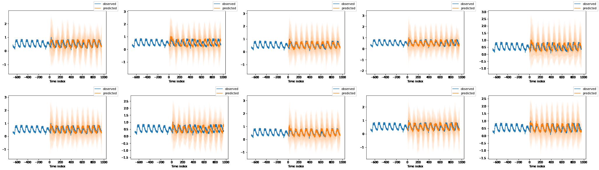
评估模型 1 2 3 4 5 6 7 best_model_path = trainer.checkpoint_callback.best_model_path best_tft = DeepAR.load_from_checkpoint(best_model_path) raw_predictions, x = best_tft.predict(val_dataloader, mode="raw" , return_x=True ) for idx in range (10 ): best_tft.plot_prediction(x, raw_predictions, idx=idx, add_loss_to_title=True );
得到了以下的几个预测图表,图表中蓝色线为旧数据,橙色为模型的预测结果。可以发现得出的预测还是看得过去的。
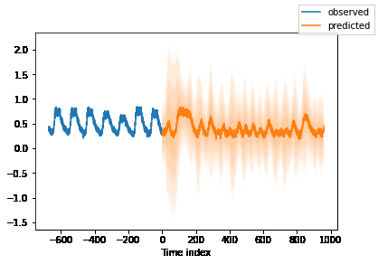
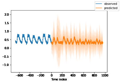
预测未来数据 1 2 3 4 5 6 7 8 9 10 11 12 13 14 15 16 17 18 19 20 21 22 23 24 25 26 27 28 29 30 31 from pytorch_forecasting import DeepARbest_model_path = "../input/the-trained-model/model.ckpt" max_prediction_length = (predicted*96 ) best_tft = DeepAR.load_from_checkpoint(best_model_path) encoder_data = summary_Table[lambda x: x.time_idx > (x.time_idx.max () - (96 *7 ))] last_data = summary_Table[lambda x: x.time_idx == x.time_idx.max ()] decoder_data = pandas.concat( [last_data.assign(summary_Table=lambda x: x.date) for i in range (1 , max_prediction_length + 1 )], ignore_index=True , ) decoder_data["time_idx" ] = decoder_data["time" ].dt.year * 12 + decoder_data["time" ].dt.month decoder_data["time_idx" ] += encoder_data["time_idx" ].max () + 1 - decoder_data["time_idx" ].min () for i in range (1 ,max_prediction_length): decoder_data["time_idx" ][i] = decoder_data["time_idx" ][i] + i decoder_data["time_idx" ] = decoder_data["time_idx" ].astype(int ) new_prediction_data = pandas.concat([encoder_data, decoder_data], ignore_index=True ) new_raw_predictions, new_x = best_tft.predict(new_prediction_data, mode="raw" , return_x=True ) miao = pandas.DataFrame(data = new_raw_predictions.prediction.numpy().tolist()[-1 ]) best_tft.plot_prediction(new_x, new_raw_predictions, idx=0 , show_future_observed=False );
1 2 3 4 5 6 7 8 9 10 11 12 # 保存预测结果到文件当中 plt.title('') plt.ylabel('load') plt.xlabel('time') plt.grid(True) plt.autoscale(axis='x', tight=True) plt.plot(miao.iloc[:,0]) # 反归一化 miao.iloc[:,0] = miao.iloc[:,0].map(lambda load: load*(max-min)+min) plt.plot(miao.iloc[:,0]) miao.to_csv("wakaka.csv")